Bayesian Inference, and Where Regularisation Comes From
Bayesian inference combines what we know before seeing the data with what the data tells us. The same framework gives two familiar tools in machine learning a probabilistic explanation. A Gaussian assumption about a model’s parameters leads to ridge regression; a Laplace assumption leads to lasso. Bayes’ theorem links them.
Introduction to Bayesian Inference
In frequentist statistics, an unknown parameter is treated as a fixed number. The data varies from one sample to the next, and probability describes that repeated sampling. Bayesian statistics instead uses a distribution to describe uncertainty about the parameter.
Bayes’ theorem explains how data and prior knowledge combine. For events and ,
The same statement holds for continuous quantities, with densities in place of probabilities, so it applies to a model’s parameters as readily as to events. Read that way it has three parts. The prior describes which parameter values are plausible before the data is seen, and is how prior knowledge about the parameters enters the model. The likelihood measures how well each value explains the observations. Their combination gives the posterior, the resulting distribution for the parameters.
The division is by the probability of the data, which is what makes the posterior integrate to one. That quantity is the same whatever the parameters are, so it cannot change which values the posterior favours. Set it aside and a single sentence is left: the posterior is proportional to the likelihood times the prior. The next section uses that sentence with priors placed directly on regression coefficients.
Bayesian Interpretation of Regularisation
Regularisation is a way to discourage a model from fitting noise in its training data. It adds a penalty to the usual measure of error, so a model must balance fitting the data against keeping its coefficients small. Ridge uses a penalty built from the squared L2 norm, found by squaring the coefficients and adding the results. Lasso uses the L1 norm, which adds their absolute values. The L1 penalty can set coefficients exactly to zero, so lasso can produce a sparse model that uses only some of the available variables.
From a machine learning point of view, the choice of squared values for ridge and absolute values for lasso can look arbitrary. Bayes’ theorem gives both penalties a source. Placing a prior on the coefficients means stating which coefficient values are plausible before seeing the data, exactly the role the prior had in the previous section. Give the coefficients a Gaussian prior centred at zero, which makes small values more plausible, ask for the peak of the posterior, and what comes out is the ridge objective, penalty and all. Give them a Laplace prior instead and out comes lasso. Neither penalty has to be added; each is already contained in the assumption. The strength of the penalty is not free either: it is fixed by how much noise the data has and how narrow the prior is, and a narrow prior, one that insists the coefficients are small, is the one that penalises heavily.
Getting from the prior to the penalty is a few lines of algebra, and if you want to see them, the linear regression chapter of Kevin Murphy’s Probabilistic Machine Learning: An Introduction works through both.
The Gaussian and the Laplace densities disagree in one place, and it is the place that decides the difference between ridge and lasso: their behaviour at zero.
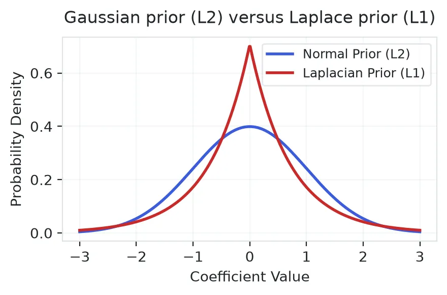
The Gaussian is smooth there. Its peak is rounded, and a rounded peak has one well-defined slope at every point on it, including at the top, where that slope is zero. Slope is what the penalty pulls with. As a coefficient gets close to zero the penalty built from the Gaussian flattens out, so the pull towards zero fades away just as the coefficient arrives. A small improvement in fit is always worth more than the vanishing amount of penalty saved by covering the last of the distance. Ridge therefore shrinks coefficients towards zero and leaves them a little short of it.
The Laplace density comes to a point. Two curves meet at zero, and they meet at a corner: approach it from the left and the slope is one value, approach from the right and it is another, and there is no single slope at the corner itself. That is what non-differentiable means here. The penalty this prior produces inherits the corner, and with it a pull towards zero that is constant, as strong at a coefficient of 0.001 as at a coefficient of 1. It never fades. A coefficient stays away from zero only while the fit it buys is worth more than that fixed cost, and when it is not, the coefficient sits at exactly zero. Sparsity is not a rule that switches variables off; it is a corner that a coefficient can settle into and has no reason to leave.
A prior records what the parameters are expected to look like before the data is seen. Applied to regression coefficients, a Gaussian prior produces ridge and a Laplace prior produces lasso. Regularisation is one consequence of putting prior knowledge on a model’s parameters and following Bayes’ theorem through.